«Introduction to autonomous mobile robots» 5.2.4 An error model for odometric position estimation
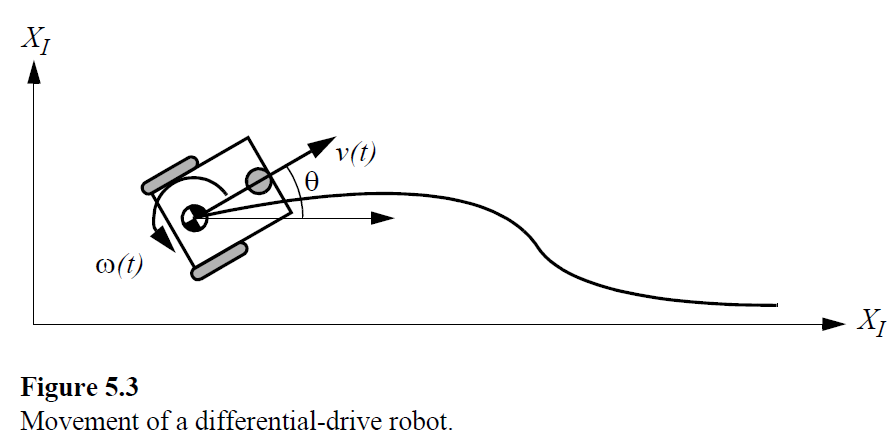
Motion model of A differential-drive robot
The pose of a robot is represented by the vector:
\[p=\left[\begin{array}{l}{x} \\ {y} \\ {\theta}\end{array}\right]\]For a discrete system with a fixed sampling interval \(\Delta t\), the incremental travel distances \((\Delta x ; \Delta y ; \Delta \theta)\) are
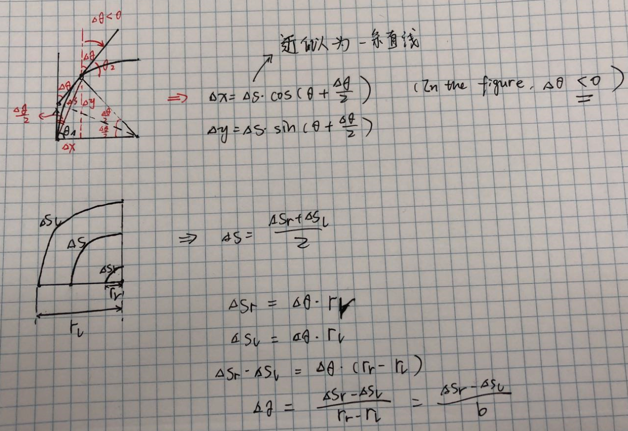
\[\Delta x=\Delta s \cos (\theta+\Delta \theta / 2),\] \[\Delta y=\Delta s \sin (\theta+\Delta \theta / 2),\] \[\Delta \theta=\frac{\Delta s_{r}-\Delta s_{l}}{b},\] \[\Delta s=\frac{\Delta s_{r}+\Delta s_{l}}{2},\]where \((\Delta x ; \Delta y ; \Delta \theta)\) = path traveled in the last sampling interval; \(\Delta s_{r} ; \Delta s_{l}\) = traveled distances for the right and left wheel respectively; \(b\) = distance between the two wheels of differential-drive robot.
Thus, we get the updated position \(p^{\prime}\):
\[p^{\prime}=\left[\begin{array}{c}{x^{\top}} \\ {y^{\prime}} \\ {\theta^{\prime}}\end{array}\right]=p+\left[\begin{array}{c}{\Delta s \cos (\theta+\Delta \theta / 2)} \\ {\Delta s \sin (\theta+\Delta \theta / 2)} \\ {\Delta \theta}\end{array}\right]=\left[\begin{array}{l}{x} \\ {y} \\ {\theta}\end{array}\right]+\left[\begin{array}{c}{\Delta s \cos (\theta+\Delta \theta / 2)} \\ {\Delta s \sin (\theta+\Delta \theta / 2)} \\ {\Delta \theta}\end{array}\right].\]Further, we obtain
\[p^{\prime}=f\left(x, y, \theta, \Delta s_{r}, \Delta s_{l}\right)=\left[\begin{array}{c}{\frac{\Delta s_{r}+\Delta s_{l}}{2} \cos \left(\theta+\frac{\Delta s_{r}-\Delta s_{l}}{2 b}\right)} \\ {\frac{\Delta s_{r}+\Delta s_{l}}{2} \sin \left(\theta+\frac{\Delta s_{r}-\Delta s_{l}}{2 b}\right)} \\ {\frac{\Delta s_{r}-\Delta s_{l}}{b}}\end{array}\right].\]Mathematical Proof